Foundations of Robotics (WIP)
[Edit]If you find any error you can edit article using edit link .
- References
- History
- Kinematics
- Motion model
- Localization
- Satellite localization
- Environment representation
- Planning
- Multirobot systems
- Satellite localization
References
- Karel Čapek: R.U.R.
- Isaac Asimov: Runaround
- B. Siciliano, O. Khatib: Handbook of Robotics
- S.M. LaValle: Planning Algorithms
- R.J. Schilling: Fundamentals of robotics: Analysis & Control
History
Robots are old and in movies. There is also robotic fish.
Prehistory
There is book Leonardos robots. Japan had mechanic dolls.
Robotic structures
- Manipulators
- 40’s of 20 century - remote manipulation with radioactive material
- 1961 - H.A. Ernst (MIT) - founder of company making manipulator robots
- Mobile robots - remotely controlled
- since ca. 70’s of 20 century
- Mobile robots - autonomous
- since ca. 90’s of 20 century
Three laws of robotics
1. Law
A robot may not injure a human being or, through inaction, allow a human being to come to harm
2. Law
A robot must obey orders given to it by human beings, except where such orders would conflict with the first law.
3. Law
A root must protect its own existence as long as such protection does not conflict with the first or second laws.
by Isaac Asimov, 1942, Runaround
Kinematics
- Motion and transformation
- translation, rotation, spherical movement
- Movement of individual robot parts without relation to forces which move it.
- Representation of the location and orientation in space
- Forward vs. Inverse kinematics
- Calculate position of end effector vs. Calculate motion to reach desired position
Degrees of freedom (DOF)
- Basic directions of translation and rotation
- 2D - 3 DOF []
- 3D - 6 DOF []
- Alternatively “ position + rotation i.r.t and planes and i.r.t. the tool rotation axis”
- Human body has 244 DOF
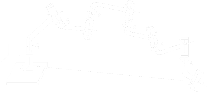
Manipulators
- Manipulation of an object in space
- at least 6 DOF for 3D
- Arms, elbows, joints, hinges
- Joint variable
- denotes joint setup, orientation
- Joints State
- DOF =
- Working space
- Local vs. Global coordinate system (LCS, GCS)
- coordinates transformation
- lokální je užitečnější
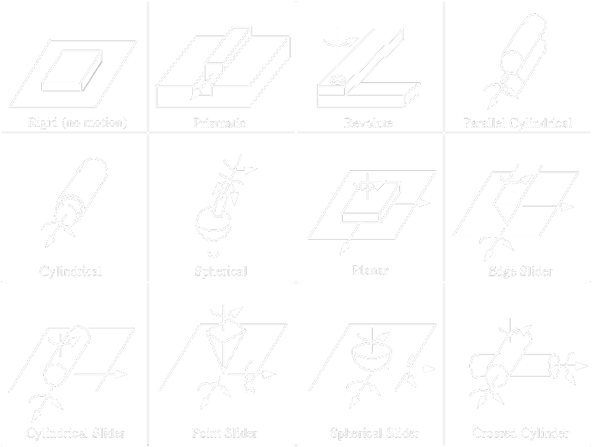
Lower pair joints
- Many variants possible, but usually:
- revolute (DOF = 1)
- prismatic (DOF = 1)
- helical (DOF = 1)
- cylindrical (DOF = 2)
- spherical (DOF = 3)
- planar (DOF = 3)
- Primitive joint types:
- prismatic
- revolute
- Most robots are build using only these two
Rotation
Rotation axis, angle
Rotation axis, angle
Rotation axis, angle
Rotation along ,, by angles , ,
Homogenní souřadnice
Bod
2D Rotation
2D Translation
Rotation + translation
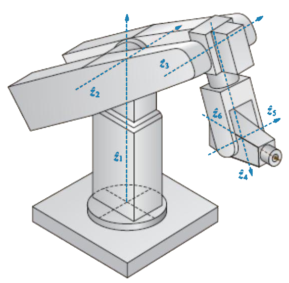
Forward kinematics (3D)
- General
- each link represented by its geometric transformation
- transition between s (local coordinates system)
- may be hard to construct the full combined transformation matrix
System composition
- General a. each link represented by its geometric transformation b. translation between s
- May be hard to construct the full combined transformation matrix
Denavit-Hartengerg
Fictive movements which connect two systems:
rotate, move, move, rotate.
That can be generalized to any sequence.
- Typical system composition
- Chains composed of rotational and translatioal joints only:
- joint connects links and
- link connects joints and
- Chains composed of rotational and translatioal joints only:
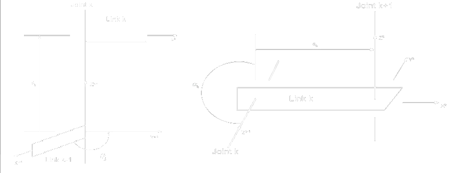
Denavit-Hartenberg overview
Definice
Relation between and is a composed transformation:
| 1. Rotate axis along by angle | |
| 2. Translate axis towards by distance | |
| 3. Translate along axis by distance | |
| 4. Rotate axis along by angle |
DH parameters:
DH transformation
-
Rotate axis along by angle
-
Translate axis towards by distance
-
Translate along axis by distance
-
Rotate axis along by angle
Finálně vše zkombinujeme
- DH parameters:
- angle between axes about (joint angle)
- distance between axes (link offset)
- distance between axes (link length)
- angle between axes about (link twist)
usage
- universal transformation between two adjacent
- Same format independent to joint type:
- Rotation - variable, others are constant
- Traslation - variable, others are constant
- Forward kinematics is easy:
- while iterating, we use always one variable and 3 constants
DH system construction
- Joints numbered ( is the first, fixed, are the rest, moving)
- Links numbered (link connects joints and )
- Right-handed orthonormal coordinate system
- Let axis be the axis of joint movement, positive direction towards positive quadrant of the basic system
- Let axis be perpendicular to and :
- and identical - endpoint of joint , parallel to
- skew share the normal a , positive direction from towards .
- intersecting perpendicular to and , in the intersection, positive direction so that it moves along from to in positive sense
- Set axis to complete the right-handed orthonormal
- Set origin at intersection of and or (if they do not intersect) at intersection of their common normal and
- Determine the four parameters:
- angle of rotation from to about
- distance from origin to along is the intersection of and (or and their common normal)
- distance from to origin along
- angle of rotation from to about
- from the endpoint of last link either parallel to or to some significant direction (e.g. supply cable)
- from the endpoint of the last link so that it intersects , positive direction towards the workspace.
Motion model
Holonomic / non-holonomic drive
Definice
A vehicle is holonomic if the number of local degrees of freedom of movement equals the number of global degrees of freedom.
Ackermann steering
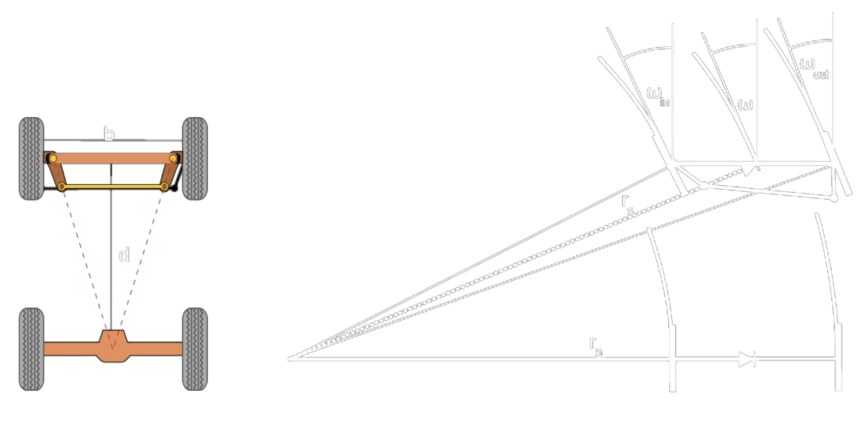 |
 |
| Basic principle | Simplified model |
- Non-holonomic
- Constant movement along a circle or straight line
- Circle:
- Orientation change
- Manoeuvring abilities depend on and (wheelbase and wheel turn)
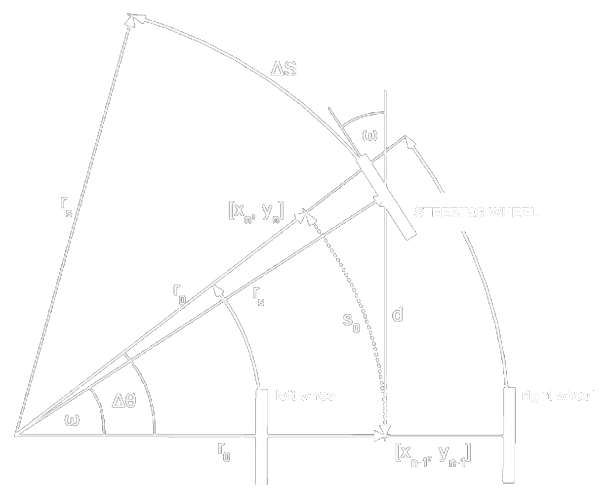
Differential steering
- non-holonomic
- Approximation:
- more precisely, integrating:
- Differential steering for real life - General trajectory is replaced by a series of
- line segments
- arcs
- Wisely set
- Odometry
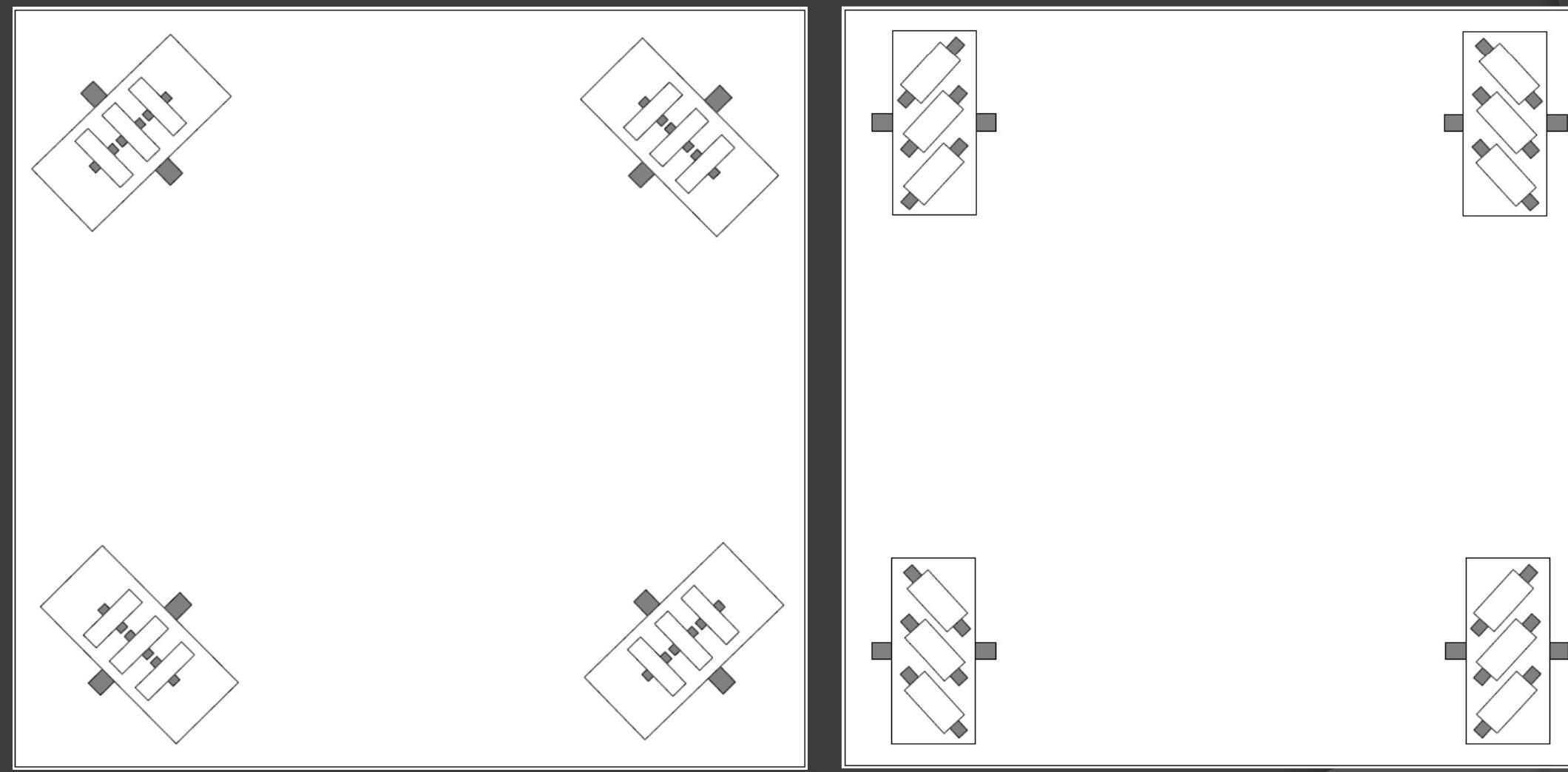
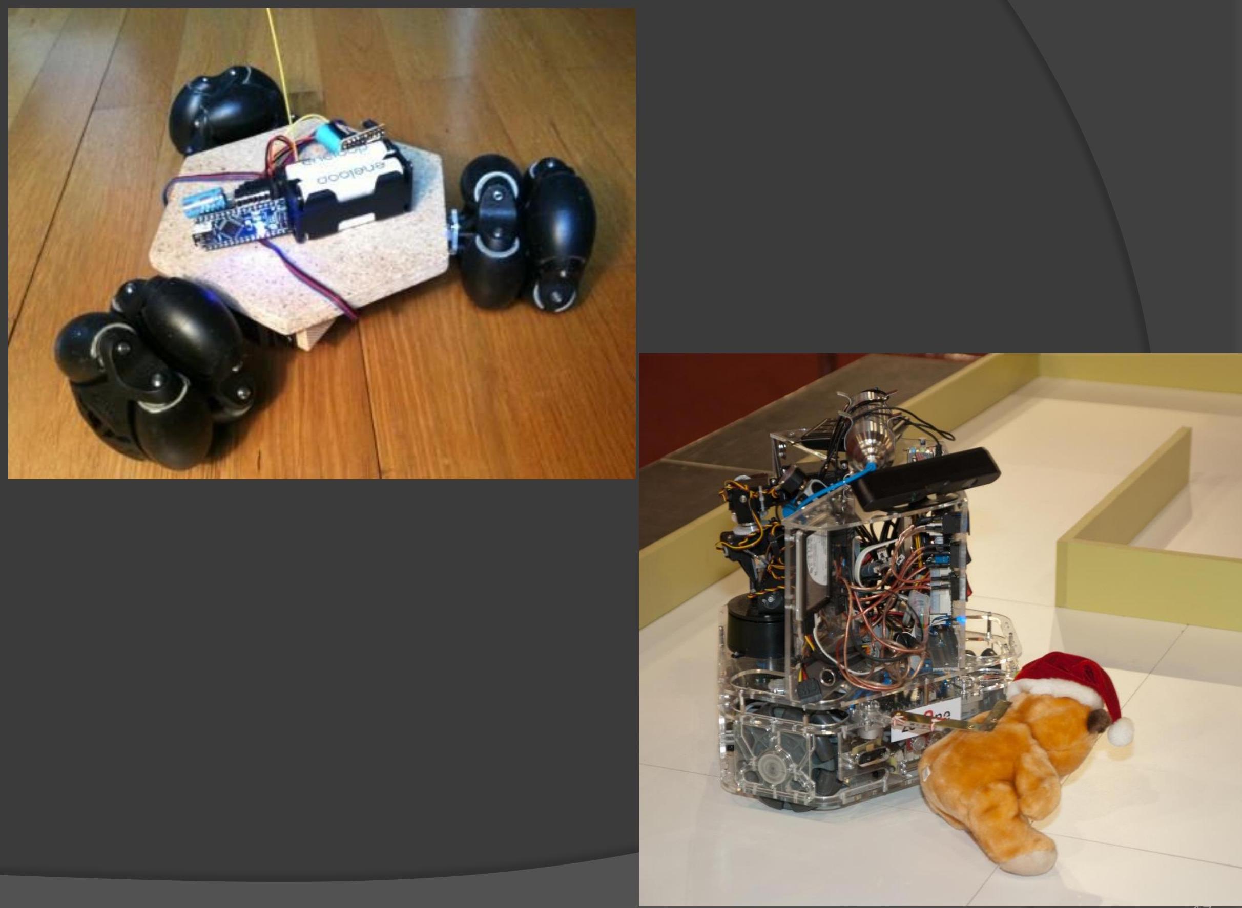
Omnidirectional steering
- Wheels are able to run in any direction
- Swerve/Crab drive
- Omniwheel
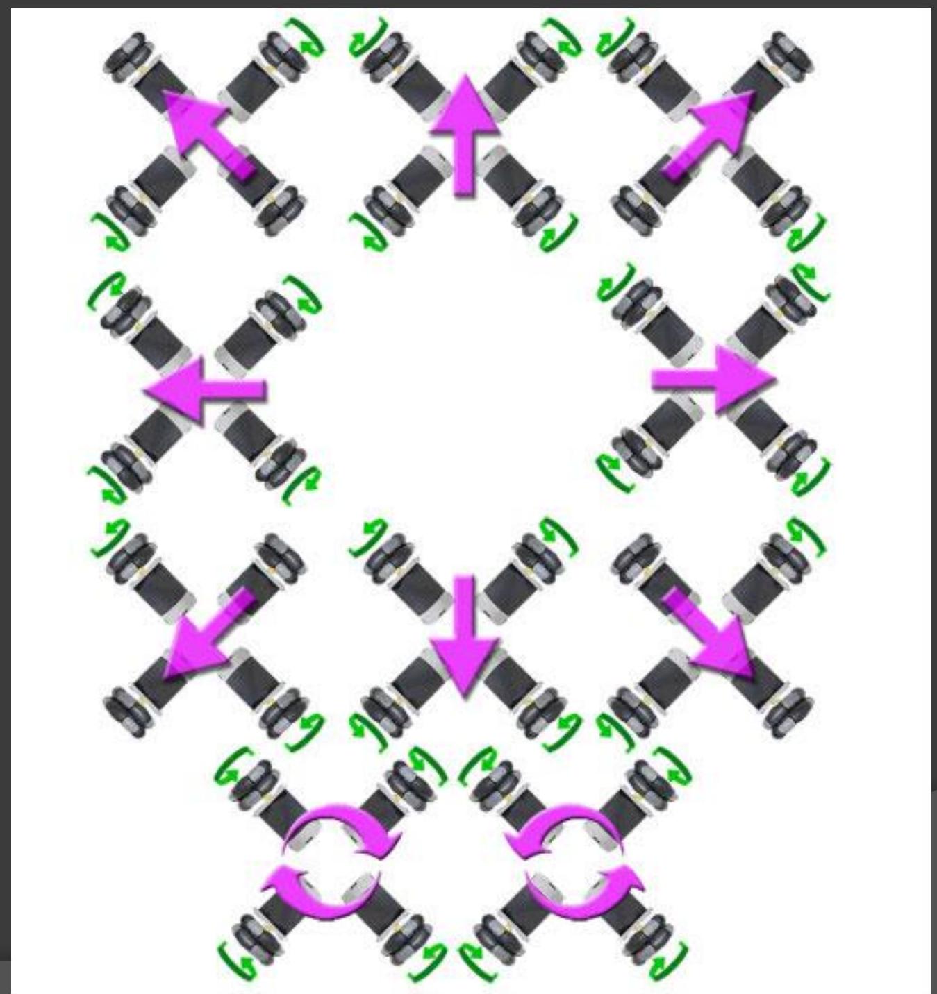
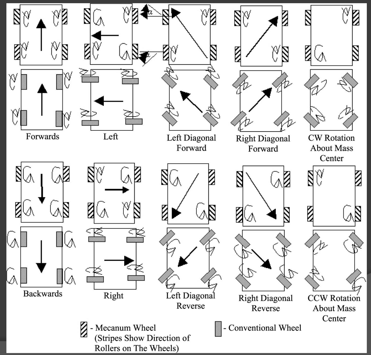
- Mecanum wheel
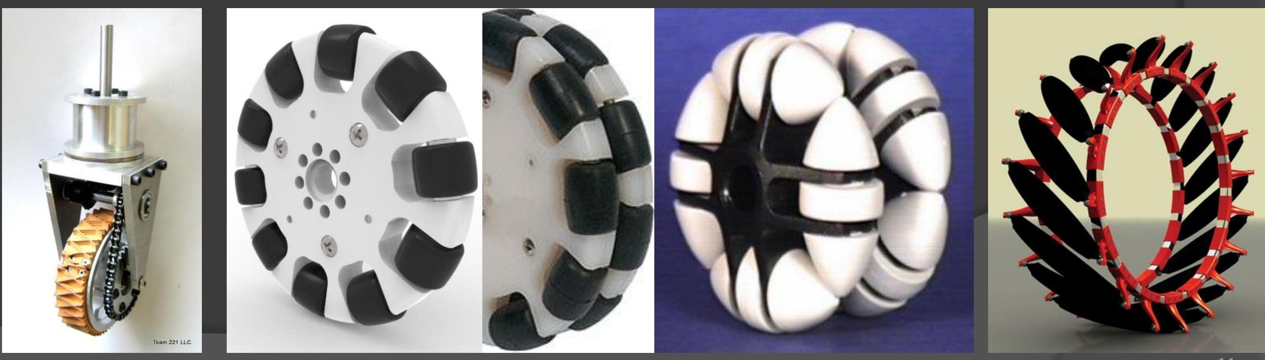 |
 |
- Syncro drive
- Holds yaw (body rotation) independently to movement direction
- Arbitrary movement as for omnidrive
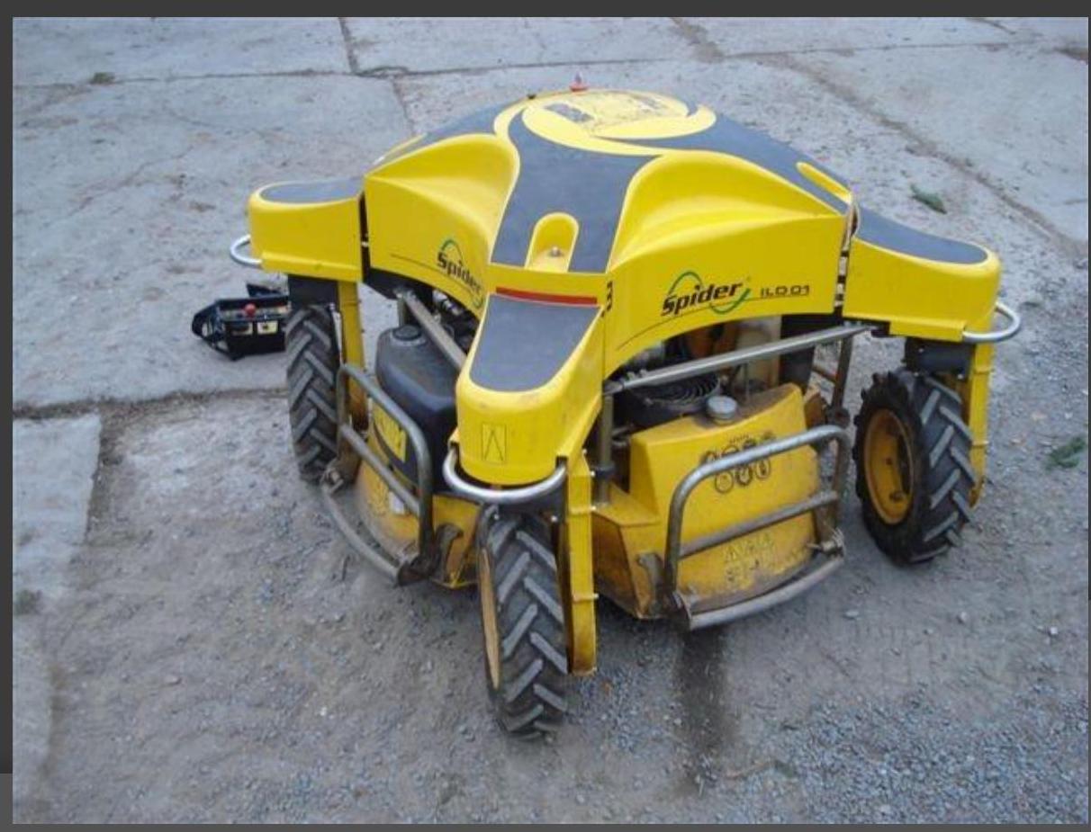
- High manoeuvring ability
- sideways run
- start in any direction
- body orientation independent on movement direction
- on-place turning
- Simpler mechanical construction for omniwheels and mecanum wheels (fixed mount)
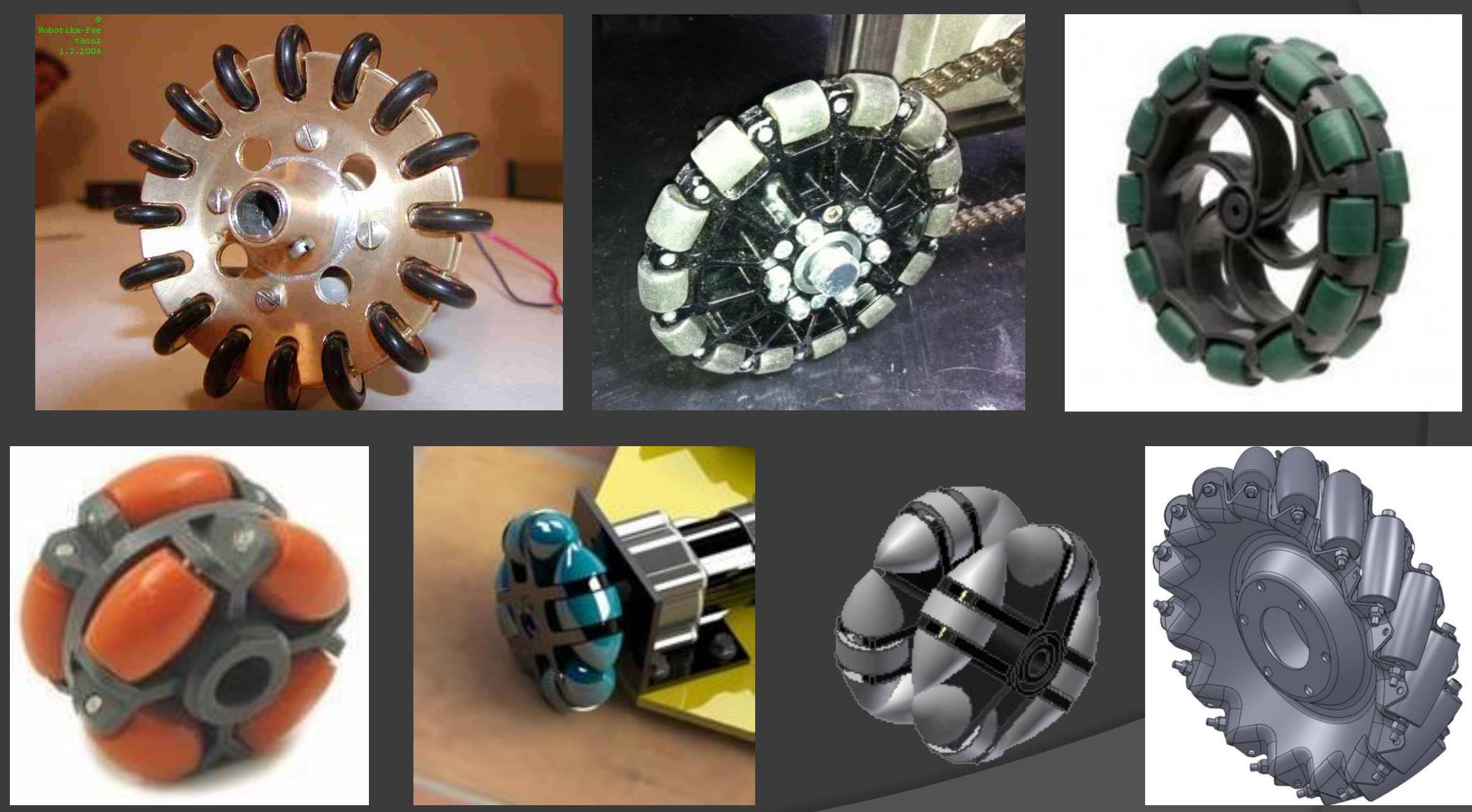
1. Holonomic
- Movement easily calculated by vector combination
2. Killough / Ilon wheels
3. Omniwheel drive
Mecanum \& swerve drive
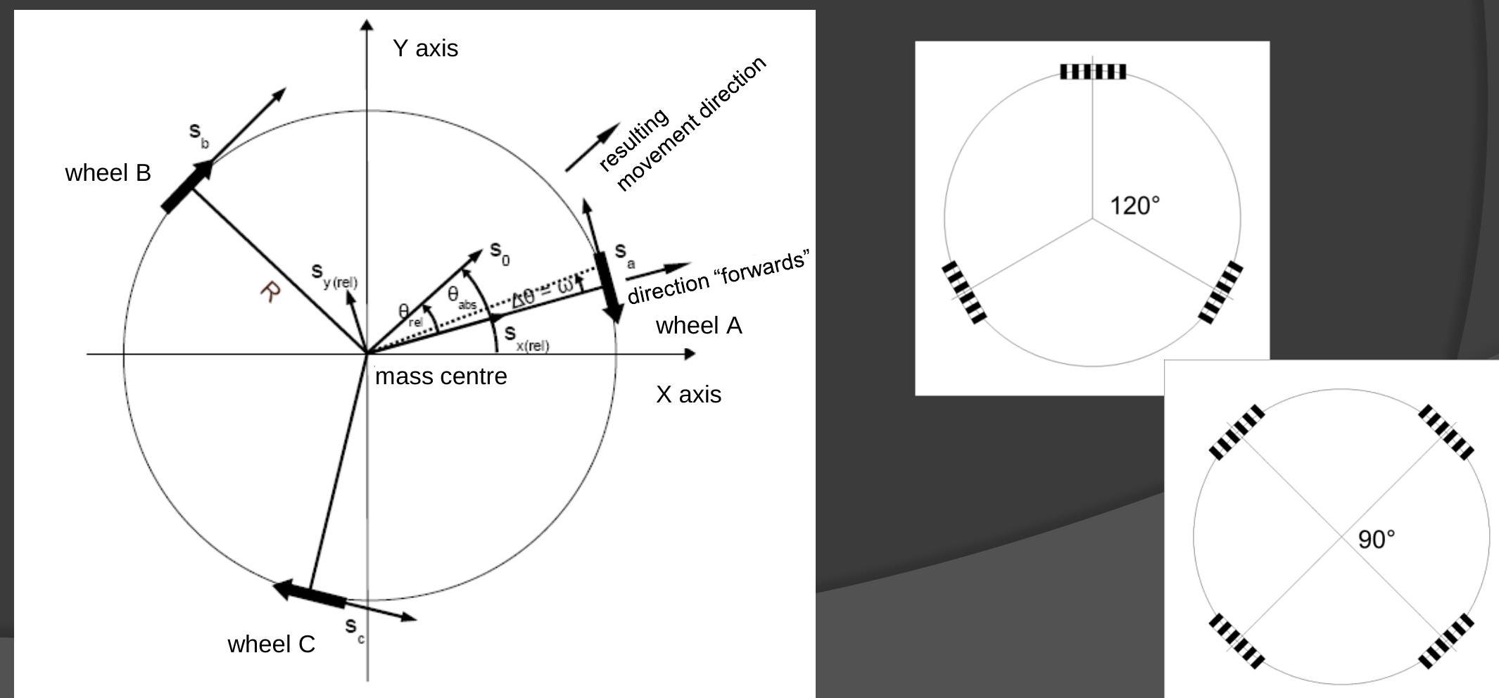
Robot movement
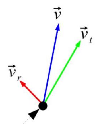
- Got (translation speed) and (rotation speeds)
- Need - specific point speed
- vector approach
 |
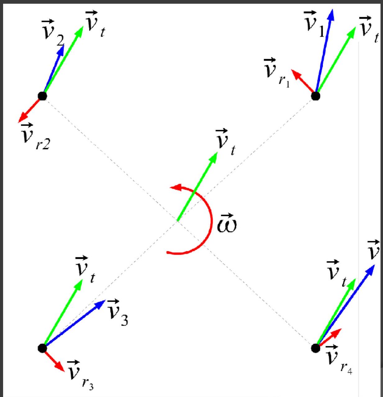 |
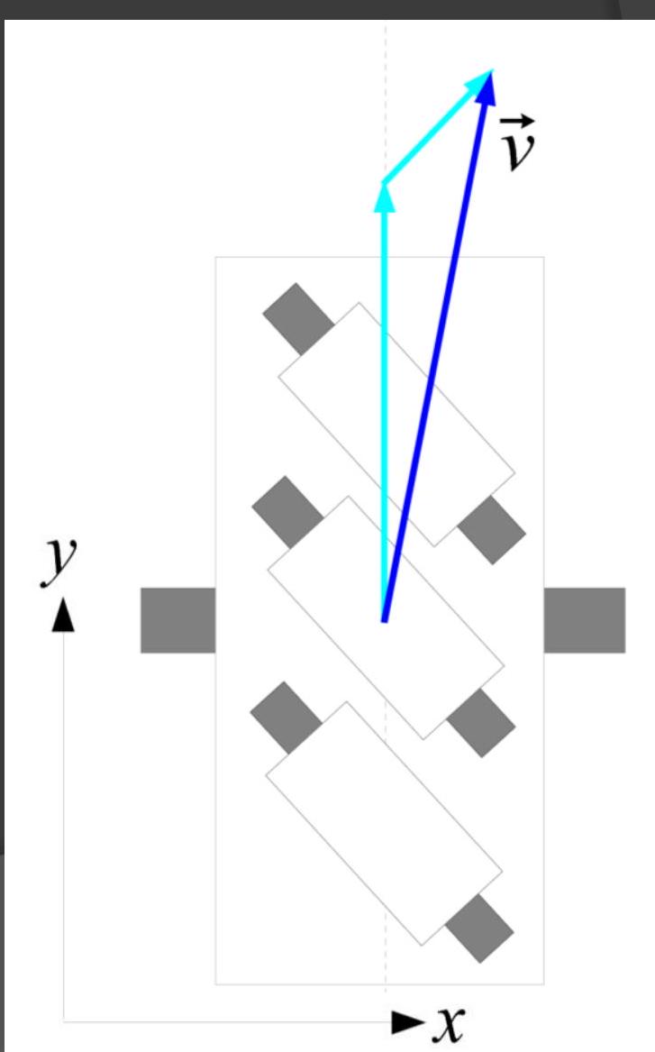
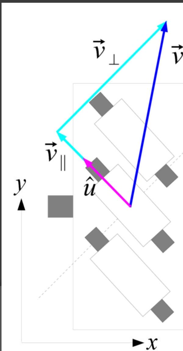
Swerve drive
- Resolve (, components = axes velocities ) into wheel speed and steering angle
- Resolve velocity into parallel and perpendicular components; magnitude of parallel component is wheel speed
- is a unit vector in the direction of the wheel (whichever direction is assumed to be “forwards”)
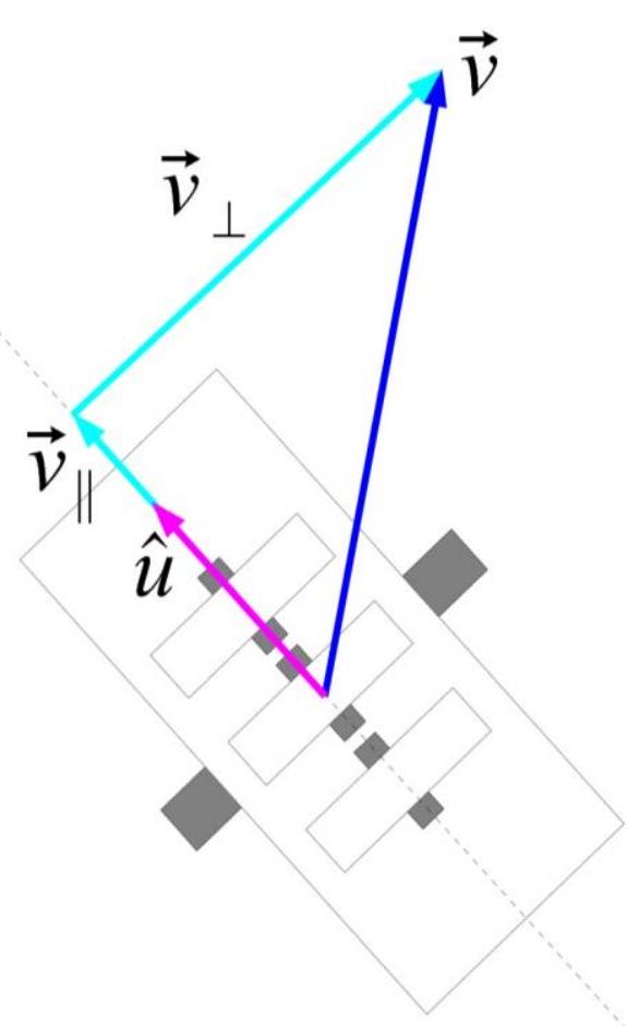
Mecanum drive
- Similar to omniwheel drive
- Conceptually: Resolve velocity into components parallel to wheel and parallel to roller
- Not easy to calculate directly (directions are not perpendicular), so do it in two steps:
- Resolve to roller
- Resolve to wheel
- Resolve velocity into components parallel and perpendicular to roller axis
- is not the same for each wheel; pick direction parallel to roller axis, in forwards direction
- Perpendicular component can be discarded
- Use component parallel to roller axis and resolve it into components parallel to wheel and parallel to roller
- is the component parallel to the wheel
- When the angle is known, we can calculate directly.
- E.g. for inclination:
Localization
- The goal is to find the position and orientation of the robot (pose)
- relative to the map
- relative to the environment
- Sometimes we also want to determine the position and orientation of individual parts
Coordinate transformation
- The map is independent of the robot’s movement
- The sensors move with the robot - it has local coordinates
- Localization tries to map the local and global position onto each other
- The pose cannot be perceived directly
- We divide localization into
- absolute (global) / relative (local)
- passive / active
- static / dynamic (lighting, obstacles,… do (not) change )
Absolute localization
- Measurement / Approximation regardless of previous state, typically more demanding on performance / technology
- Localization after reset / relocation is problematic (wake up / kidnap problem)
- Uses landmarks, or GPS and other services
Relative localization
- Track position and update (odometry)
- we know the initial position
- we measure / estimate the change compared to the previous state (change in rotation and orientation)
- The problem is the accumulation of the error - after a long time the error can be too large
Dead reckoning
- the easiest localization
- direction + speed + time of movement
- accumulates an error
Odometry
- Measurement of wheel rotation (in different places we measure slightly different values) (TODO to explain)
- Systematic errors:
- losses
- different wheel radii
- other specified and actual parameters
- asymmetry
- measurement resolution
- sampling frequency
- etc.
- Unsystematic errors:
- terrain irregularities
- obstacles
- poor contact with the surface
Robot centric sensors
Most sensors move with the robot, so we have to do further data processing (e.g. recalculate coordinates relative to the global system,).
Types of localization
- Passive
- does not affect the control of the robot
- Active localization
- If the measurement is needed, it will affect the behavior of the robot
- active measurement and navigation
- Realistic localization
- Inputs are not trustworthy, actuators are not reliable, external influences must be taken into account
A possible solutions
- More accurate measurement - better sensors and actuators, data filtering, the most accurate model of the robot and the environment
- Do not rely on the fact that localization is accurate - probabilistic methods, fuzzy logic, interval algebra
- We can consider the data as random variables (inputs, pose)
- The position estimate is then a distribution
- Localization is then the search for a distribution that best matches the real position of the robot
- In 1D Belief where Ideally, for exact but we can’t reach the position
- We want to model
- Random modeling can be used with particle filters, Bayesian methods,…
- We estimate the posterior by measuring the prior
Representation
- Continuous representation is more accurate but harder to obtain and maintain (Kalman filter)
- That’s why we use a rather discrete representation
- This way we get probability grids, topological graphs,…
Probability Grid
- indicates the probability of the appearance of a robot in the field
- Difficulty depends on grid fineness and map size
- It can be reduced using
- selective updates (only interesting part of the grid)
- Hierarchical models (quadtree)
- non-orthogonal graphs
Topological graphs
- Nodes - positions, edges - possible transitions
- indicates the probability of occurrence in a given node
- More nodes can be made in the place where the robot is more likely to be found
- The chart does not need to contain geometric data
Monte Carlo localization
- A set of weighted points in space
- is the sum of the weights of points at a given distance from l
- More points can be created for a more likely location
- Algorithm:
- Sample movement, weights do not change
- Correction, the positions of the points do not change, recalculate the weights
- Oversampling, cleaning - discard unnecessary points, add new ones,…
- Doesn’t work well for too accurate sensors, but not too imprecise either
- There is a lot of noise when navigating outside - MC can combine multiple measurements well
Continuous representation (Kalman filter)
- based on a normal distribution
- cannot record multiple hypotheses
- strict assumption: measurements must have a normal distribution
Other methods
- fuzzy logic
- interval algebra
Solution 3 no localization
- hardcoded automata
- reactive systems
- evolutionary algorithms
SLAM
- simultaneous location and mapping
- browsing a static environment
- we want to create a map and find the position from it
- a poorly recognized landmark can cause a huge error
- when using more landmarks, the difficulty increases (, with improvements)
- map errors and movement errors can be correlated
- knowledge of the angle with respect to two landmarks determines the part of the circle
- in addition, the distance can be calculated while moving
Satellite localization
If we know the distance of the aiming point from the satellite, it will determine the sphere. Two specifies a circle and three a point. In practice, at least four satellites are typically used.
Simple idea: measuring the signal time-of-flight distance
History
- Werner von Braun (V1, V2,…)
- Sputnik(1957) The Doppler effect on the signal was another idea for a method of measurement.
- Transit
- US Navy
- proof of concept, but didn’t cover the whole country, slow, 2D only
- TODO technology
- Timeation
- uses precise (later atomic) clocks
- 2D only
- 621B
- US air force
- Can also target planes (3D)
- Pseudo-random noise increases resilience
- Needs constant satellite-ground connection
- NAVSEG
- a group formed by the cooperation of several sectors
- Uses ideas from Transit (orbit + prediction) and Timetion (accurate clock) and 621B (resilient signal)
- In 1973, Navstar GPS was created, the basis of today’s GPS launched in 1978
- Accuracy about 10 m
- Initially intended only for the military, later a less accurate version of the signal was broadcast for civilian purposes.
- Since 2000, even the more accurate army version is available to everyone
- Navigation failure caused several air accidents (typically wrong trajectory -> shot down USSR)
GPS satellites
- 6 Orbit gap declination after four slots
- There are at least four satellites in each orbit
- At least 4 satellites are visible from every location on earth
- Due to atmospheric phenomena and calculation errors, the GPS error is about 15m with post processing, better accuracy around 10m can be achieved
Competitive global systems
Compass(China), Galileo(EU), GLONASS(Russia)
Regional systems
Beidou(China), DORIS(France), IRNSS(India)
Local systems
- EGNOS, GAGAN, MSAS, WAAS
- Typically a stationary satellite
Galileo
European project, more accurate (about 1 m)
Ublox
- centimeter accuracy
- uses RTK technology, which combines several techniques and thus achieves higher accuracy (verify)
Indoor GPS
- Local location determination can be done using Wifi or bluetooth
- More accurate technology can achieve about 1m accuracy
Environment representation
Maps
we divide according to several aspects
- according to production
- manual (expensive)
- (semi)automatic
- According to production time
- online
- offline
- According to time of use
- Firm
- adaptive
- basic division
- Metric
- Topological
- By level of abstraction
- Sensory
- Geometric
- Topological
- Symbolic
Types of maps
- Metric maps
- Based on the given coordinate system
- Objects are represented by coordinates
- tourist map, (city plan)…
- Topological maps
- They don’t have positional information only about relationships between objects.
- For example connections, neighboring objects…
- Additional information: names, attributes and other data important to the robot.
- Typically chart + labels + metadata.
- Maps in robotics tend to be a combination of both approaches.
- Sensory maps
- Uses sensor input or pre-processed data (filtered,…).
- For example occupancy grid - regular (square, hex,…) or irregular (various sizes and shapes).
- Mostly they are only local
- Geometric maps
- Description based on geom objects: curves, cubes, cylinders,…
- Automatic production is demanding
- Topological maps
- typically a geom map generalized to a graph
- mostly used by:
- nodes = objects and edges = adjacent obj
- nodes = objects and connections, edges = affiliations (TODO meaning)
- Symbolic maps
- for direct robot communication with people, e.g. prolog(?)
- Occupancy grid
- directly it is difficult to maintain
- probabilistic methods
- fuzzy approach
- Neurons, genetic alg. - a problem with learning and anticipating unexpected events
- directly it is difficult to maintain
Planning
Prerequisites
- Mapping
- Knowledge of location and destination
- Movement model
- Metric
Description of the problem
- go from start to finish
- find a path or notice that it does not exist
- reacts to the surroundings - avoiding obstacles,…
- Sometimes we want navigation: planning and avoiding obstacles
- Planning is the opposite of avoiding obstacles, however both complement each other
Scheduling algorithms
- Graph methods
- Use of grid, potential field
- independent of map type
- Exact, Approximate, Probabilistic,
Bug algorithm
- has no global model - no map, does not know the location of obstacles or if there is a solution
- knows the destination location relative to the starting location
- only local detection of the surroundings (contact), possibly at a short distance
- Reactive
Prerequisites bug alg
- 2D static environment
- Final parameters: the number of obstacles and their perimeters,
- non-zero thickness of obstacles
- Straight line crosses with obstacles
- Obstacles do not touch, they can be united when overlapping
Bug 0
- Go straight to the target
- When you hit an obstacle, go around the obstacle until you can’t go straight to the goal
- It may not work - for example, for a circle with a small hole (where the target is on the opposite side to the center), the robot will go inside and before it comes out, it will get to the state where it can go to the target again
Bug 1
- Go straight to the target
- When you hit an obstacle, go around the obstacle
- After you go around the obstacle, go to the place that was closest to the goal and go straight again
- The robot will never return to the obstacle from which it left (it will exit from the place that is closest to the target towards it)
- Because the robot’s position is always in a sufficiently large circle around the target, it will encounter only finitely many obstacles, so the algorithm is finite.
- The robot does not ignore obstacles, so the paths found are valid
- If the path existed but the robot did not find it, then the path from the minimum to the goal must lead directly to the obstacle
-
But each straight line passes through the obstacle times. Therefore there is another intersection, this intersection must be closer to the goal because it lies on the way to the goal. If there is a path to this place, the robot would choose this - the dispute cannot get closer to the goal. (TODO check)
- Distance Estimate
- Best case
- Worst case
- For each obstacle in the circle from the target, we count 1.5 times the perimeter (he goes around it and chooses a shorter path to the minimum) +
Bug 2
Go to the goal, if you come across an obstacle, go around it until you can’t go straight to the goal again
Lemma
Bug 2 finally encounters many obstacles and passes them all through the start-finish junction
Bug 2 passes each point on the obstacle at most times, where is the number of crossings of the obstacle with the start-finish line.
- Distance Estimate
- Best case
- Worst case - For each obstacle on the connecting line between the start and the finish line, we count half the circumference
Comparison of Bug 1 and Bug 2 (TODO)
There are cases for which 1 is better than two and vice versa
Estimates for length can be improved if the robot can see some of its surroundings (area inside the circle around itself)
Tangent bug
selects by angle of direction to direction to target (TODO) It is correct
Dijkstra
alternative path search A* is a Dijkstra + heuristic, if the heuristic satisfies something it can be proven that it does not process vertices twice. E.g. price + distance from destination D* also handles replanning when an obstacle appears, starting from the destination
Rapidly exploring random trees
Randomized algorithm It quickly finds some solution and iteratively adjusts
Potential field
The robot is in sweat. fields, obstacles are peaks - repel the goal is the minimum
Multirobot systems
Why use multirobot systems
- Too challenging for one robot
- The task is naturally distributed
- One universal robot would be too complex, more specialized ones are easier to make
- Parallelism accelerates the solution of the task
- Greater robustness
- Application
- Warehouses
- Modeling the real world
- A swarm of robots
- robots can cooperate or act independently
Types of systems
- Centralized Architecture
- One control center
- Possible but problematic: the failure of the center may mean the failure of all robots, too much communication load on the center.
- Hierarchical Architecture
- Divide and rule
- Robots have small groups of robots that he gives orders to
- Scales better, problematic when higher level control fails
- Decentralized Architecture
- robots act according to (semi) local perceptions
- Every robot must know high level target, problematic target changes
- Hybrid driving
- combination of local control with control of multiple robots (TODO check)
Satellite localization
If we know the distance of the aiming point from the satellite, it will determine the sphere. Two specifies a circle and three a point. In practice, at least four satellites are typically used.
Simple idea: measuring the signal time-of-flight distance
History
- Werner von Braun (V1, V2,…)
- Sputnik(1957) The Doppler effect on the signal was another idea for a method of measurement.
- Transit
- US Navy
- proof of concept, but didn’t cover the whole country, slow, 2D only
- TODO technology
- Timeation
- uses precise (later atomic) clocks
- 2D only
- 621B
- US air force
- Can also target planes (3D)
- Pseudo-random noise increases resilience
- Needs constant satellite-ground connection
- NAVSEG
- a group formed by the cooperation of several sectors
- Uses ideas from Transit (orbit + prediction) and Timetion (accurate clock) and 621B (resilient signal)
- In 1973, Navstar GPS was created, the basis of today’s GPS launched in 1978
- Accuracy about 10 m
- Initially intended only for the military, later a less accurate version of the signal was broadcast for civilian purposes.
- Since 2000, even the more accurate army version is available to everyone
- Navigation failure caused several air accidents (typically wrong trajectory shot down USSR)
GPS satellites
- 6 Orbit gap declination after four slots
- There are at least four satellites in each orbit
- At least 4 satellites are visible from every location on earth
- Due to atmospheric phenomena and calculation errors, the GPS error is about 15m with post processing, better accuracy around 10m can be achieved
Competitive global systems
Compass(China), Galileo(EU), GLONASS(Russia)
Regional systems
Beidou(China), DORIS(France), IRNSS(India)
Local systems
- EGNOS, GAGAN, MSAS, WAAS
- Typically a stationary satellite
Galileo
European project, more accurate (about 1 m)
Ublox
- centimeter accuracy
- uses RTK technology, which combines several techniques and thus achieves higher accuracy (verify)
Indoor GPS
- Local location determination can be done using Wifi or bluetooth
- More accurate technology can achieve about 1m accuracy