Probability
Experiments & Sample Spaces
- Experiment, process, test, …
- Set of possible basic outcomes: sample space Ω
- coin toss (Ω={head, tail}), die (Ω={1,…,6})
- yes/no opinion poll, quality test (bad/good) (Ω={0,1})
- lottery (∣Ω∣≅107…1012)
- # of traffic accidents somewhere per year (Ω=N)
- spelling errors ( Ω=Z∗ ), where Z is an alphabet, and Z∗ is a set of possible strings over such an alphabet
- missing word (∣Ω∣≅vocabulary size )
Events
- Event A is a set of basic outcomes
- Usually A⊆Ω, and all A∈2Ω (the event space)
- Ω is then the certain event, ∅ is the impossible event
- Example:
- experiment: three times coin toss
- Ω={HHH,HHT,HTH,HTT,THH,THT,TTH,TTT}
- count cases with exactly two tails: then A={HTT,THT,TTH}
- all heads: A={HHH}
Probability
- Repeat experiment many times, record how many times a given event A occurred (“count” c1 ).
- Do this whole series many times; remember all ci.
- Observation: if repeated really many times, the ratios of ci/Ti (where Ti is the number of experiments run in the i-th series) are close to some (unknown but) constant value.
- Call this constant a probability of A. Notation: p(A)
Estimating probability
- Remember: … close to an unknown constant.
- We can only estimate it:
- from a single series (typical case, as mostly the outcome of a series is given to us and we cannot repeat the experiment), set
p(A)=c1/T1.
- otherwise, take the weighted average of all ci/Ti (or, if the data allows, simply look at the set of series as if it is a single long series).
- This is the best estimate.
Example
- Recall our example:
- experiment: three times coin toss
- Ω={HHH,HHT,HTH,HTT,THH,THT,TTH,TTT}
- count cases with exactly two tails: A={HTT,THT,TTH}
- Run an experiment 1000 times (i.e. 3000 tosses)
- Counted: 386 cases with two tails (HTT, THT, or TTH)
- estimate: p(A)=386/1000=.386
- Run again: 373, 399, 382, 355, 372, 406, 359
p(A)=.379 (weighted average) or simply 3032/8000
- Uniform distribution assumption: p(A)=3/8=.375
Basic Properties
- Basic properties:
- p: 2Ω→[0,1]
- p(Ω)=1
- Disjoint events: p(∪Ai)=∑ip(Ai)
- [NB: axiomatic definition of probability: take the above three conditions as axioms]
- Immediate consequences:
p(∅)p(Aˉ)a∈Ω∑p(a)=0=1−p(A),A⊆B⇒p(A)≤p(B)=1
Joint and Conditional Probability
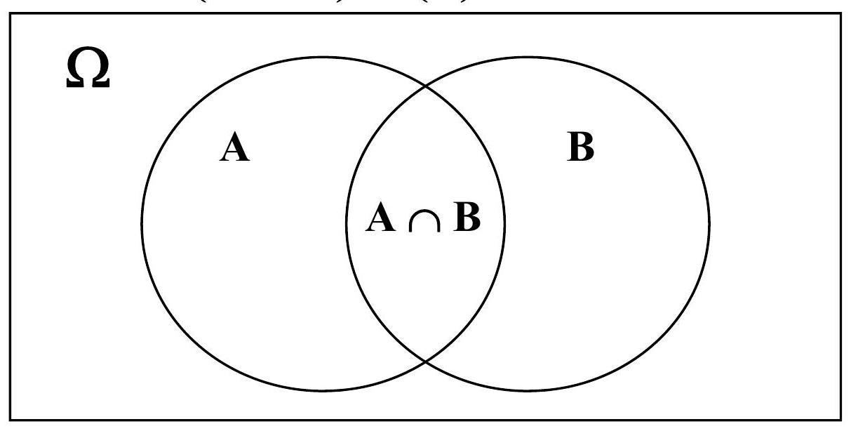
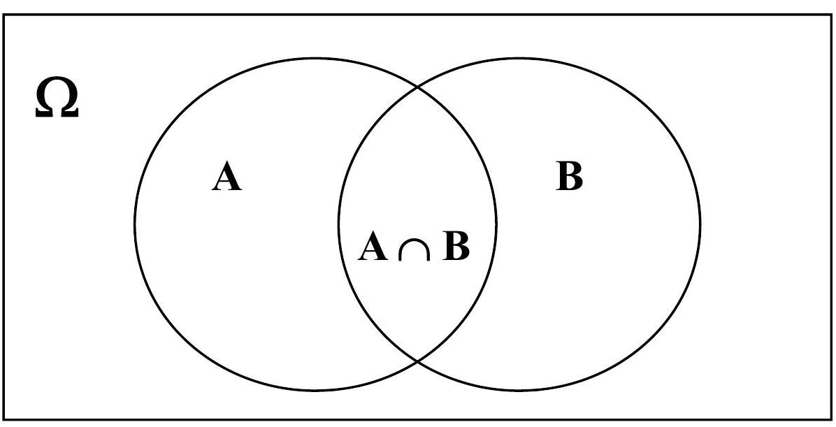
p(A,B)=p(A∩B)
p(A∣B)=p(A,B)/p(B)
Estimating from counts:
p(A∣B)=p(A,B)/p(B)=(c(A∩B)/T)/(c(B)/T)=c(A∩B)/c(B)

Bayes Rule
p(A,B)=p(B,A)
since
p(A∩B)=p(B∩A)
therefore
p(A∣B)p(B)=p(B∣A)p(A)
and therefore
p(A∣B)=p(B∣A)p(A)/p(B)

Independence
- Can we compute p(A,B) from p(A) and p(B)?
- Recall from previous foil:
p(A∣B)p(A∣B)p(B)p(A,B)=p(B∣A)p(A)/p(B)=p(B∣A)p(A)=p(B∣A)p(A)
… we’re almost there: how p(B∣A) relates to p(B)?
p(B∣A)=p(B) (iff A and B are independent)
- Example: two coin tosses, weather today and weather on March 4th, 1789;
- Any two events for which p(B∣A)=p(B)!
Chain Rule
p(A1,A2,A3,A4,…,An)=
p(A1∣A2,A3,A4,…,An)×p(A2∣A3,A4,…,An)×
×p(A3∣A4,…,An)×…×p(An−1∣An)×p(An)
- Also applicable for conditional probabilities.
- Basic idea: instead of estimating a complex joint distribution, break it up into the products of simpler conditional distributions.
Bayesian Network
- A Bayesian network (or belief network) is a graphical model that represents a set of variables and their conditional dependencies via a directed acyclic graph (DAG).
Total Probability Law
- Sum up conditional probabilities:
p(A)=i∑p(A,Bi)=i∑p(A∣Bi)p(Bi)
Normalization
- Let’s sum up over all possible outcomes:
p(Ω)ω∑p(ω)ω∑p(ω∣B)p(B)ω∑p(ω∣B)=1=1=1 for any B =1 for any B
- i.e. conditional probabilities of a variable given a value of another variable sum up to 1.
Markov Assumption
- Graphical representations of p(x1,x2,…,xn) often decompose the overall distribution into locally conditioned distributions.
- Simplest decomposition (often very accurate for natural processes): the value of xt is (conditionally) dependent only on the value of xt−1, i.e.
p(x1,x2,…,xn)=p(x1)t=2∏np(xt∣xt−1)
- (this is often called the first order Markov model or Markov chain)
- N-th order Markov models: xt conditionally dependent on xt−1,xt−2,…,xt−n :
p(x1,x2,…,xn)=p(x1,x2,…,xn)t=n+1∏Tp(xt∣xt−1,xt−2,…,xt−n)


